bigglm on your big data set in open source R, it just works - similar as in SAS
In a recent post by Revolution Analytics (link & link) in which Revolution was benchmarking their closed source generalized linear model approach with SAS, Hadoop and open source R, they seemed to be pointing out that there is no 'easy' R open source solution which exists for building a poisson regression model on large datasets.
This post is about showing that fitting a generalized linear model to large data in R <is> easy in open source R and just works.
For this we recently included bigglm.ffdf in package ffbase to integrate it more closely with package biglm. That was pretty easy as the help of the chunk function in package ff already shows how to do it and the code in the biglm package is readily available to do some simple code modifications.

Let's show how it works on some readily available data available here.
The following code shows some features (laf_open_csv, read.csv.ffdf, table.ff, binned_sum.ff, biglm.ffdf, expand.ffgrid and merge.ffdf) of package ffbase and package ff which can be used in a standard setting where you have your large data, want to profile it, see some bivariate statistics and build a simple regression model to predict or understand your target.
It imports a flat file in an ffdf, shows some univariate statistics, does a fast group by and builds a linear regression model.
All without RAM problems as the data is in ff.
- Download the data
require(ffbase)
require(LaF)
require(ETLUtils)

download.file("http://www.cms.gov/Research-Statistics-Data-and-Systems/Statistics-Trends-and-Reports/BSAPUFS/Downloads/2010_Carrier_PUF.zip", "2010_Carrier_PUF.zip")
unzip(zipfile="2010_Carrier_PUF.zip")
- Import it (showing 2 options - either by using package LaF or with read.csv.ffdf using argument transFUN to recode the input data according to the codebook which you can find here)
## the LaF package is great if you are working with fixed-width format files but equally good for csv files and laf_to_ffdf does what it
## has to do: get the data in an ffdf
dat <- laf_open_csv(filename = "2010_BSA_Carrier_PUF.csv",
  column_types = c("integer", "integer", "categorical", "categorical", "categorical", "integer", "integer", "categorical", "integer", "integer", "integer"),
  column_names = c("sex", "age", "diagnose", "healthcare.procedure", "typeofservice", "service.count", "provider.type", "servicesprocessed", "place.served", "payment", "carrierline.count"),
  skip = 1)
x <- laf_to_ffdf(laf = dat)

## the transFUN is easy to use if you want to transform your input data before putting it into the ffdf,
## it applies a function to your read input data which is read in in chunks
## We use it here to recode the numbers to factors according to the code book which you can find in the codebook
x <- read.csv.ffdf(file = "2010_BSA_Carrier_PUF.csv",
                   colClasses = c("integer","integer","factor","factor","factor","integer","integer","factor","integer","integer","integer"),
                   transFUN=function(x){
  names(x) <- recoder(names(x),
                      from = c("BENE_SEX_IDENT_CD", "BENE_AGE_CAT_CD", "CAR_LINE_ICD9_DGNS_CD", "CAR_LINE_HCPCS_CD",
                                  "CAR_LINE_BETOS_CD", "CAR_LINE_SRVC_CNT", "CAR_LINE_PRVDR_TYPE_CD", "CAR_LINE_CMS_TYPE_SRVC_CD",
                                  "CAR_LINE_PLACE_OF_SRVC_CD", "CAR_HCPS_PMT_AMT", "CAR_LINE_CNT"),
                      to = c("sex", "age", "diagnose", "healthcare.procedure",
                             "typeofservice", "service.count", "provider.type", "servicesprocessed",
                             "place.served", "payment", "carrierline.count"))
  x$sex <- factor(recoder(x$sex, from = c(1,2), to=c("Male","Female")))
  x$age <- factor(recoder(x$age, from = c(1,2), to=c("Under 65", "65-69", "70-74", "75-79", "80-84", "85 and older")))
  x$place.served <- factor(recoder(x$place.served,
                                   from = c(0, 1, 11, 12, 21, 22, 23, 24, 31, 32, 33, 34, 41,
                                            42, 50, 51, 52, 53, 54, 56, 60, 61, 62, 65, 71, 72,
                                            81, 99),
                                   to = c("Invalid Place of Service Code", "Office (pre 1992)",
                                          "Office","Home","Inpatient hospital","Outpatient hospital",
                                          "Emergency room - hospital","Ambulatory surgical center","Skilled nursing facility",
                                          "Nursing facility","Custodial care facility","Hospice","Ambulance - land","Ambulance - air or water",
                                          "Federally qualified health centers",
                                          "Inpatient psychiatrice facility", "Psychiatric facility partial hospitalization",
                                          "Community mental health center", "Intermediate care facility/mentally retarded",
                                          "Psychiatric residential treatment center", "Mass immunizations center",
                                          "Comprehensive inpatient rehabilitation facility",
                                          "End stage renal disease treatment facility",
                                          "State or local public health clinic","Independent laboratory", "Other unlisted facility")))
  x
  }, VERBOSE=TRUE)
class(x)
dim(x)
- Profile your data
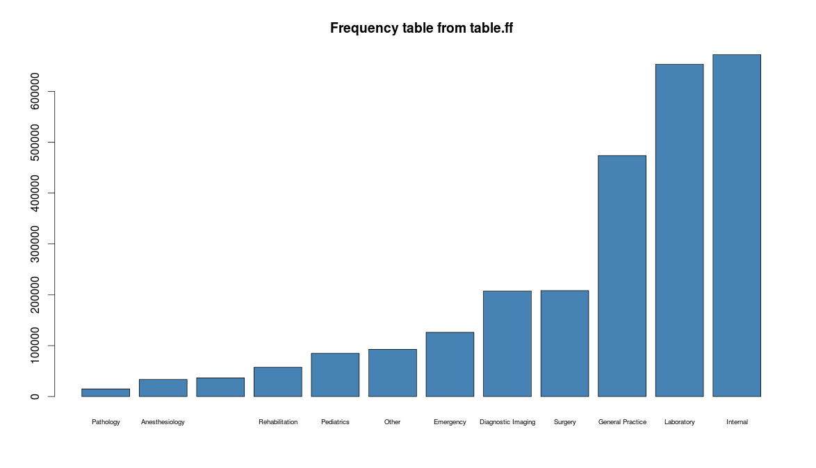
##
## Data Profiling using table.ff
##
table.ff(x$age)
table.ff(x$sex)
table.ff(x$typeofservice)
barplot(table.ff(x$age), col = "lightblue")
barplot(table.ff(x$sex), col = "lightblue")
barplot(table.ff(x$typeofservice), col = "lightblue")
- Grouping by - showing the speedy binned_sum
##
## Basic & fast group by with ff data
##
doby <- list()
doby$sex <- binned_sum.ff(x = x$payment, bin = x$sex, nbins = length(levels(x$sex)))
doby$age <- binned_sum.ff(x = x$payment, bin = x$age, nbins = length(levels(x$age)))
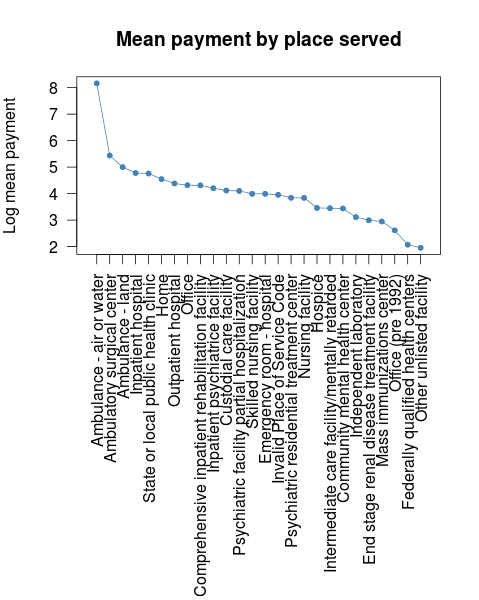
doby$place.served <- binned_sum.ff(x = x$payment, bin = x$place.served, nbins = length(levels(x$place.served)))
doby <- lapply(doby, FUN=function(x){
x <- as.data.frame(x)
x$mean <- x$sum / x$count
x
})
doby$sex$sex <- recoder(rownames(doby$sex), from = rownames(doby$sex), to = levels(x$sex))
doby$age$age <- recoder(rownames(doby$age), from = rownames(doby$age), to = levels(x$age))
doby$place.served$place.served <- recoder(rownames(doby$place.served), from = rownames(doby$place.served), to = levels(x$place.served))
doby
- Build a generalized linear model using package biglm which integrates with ffbase::bigglm.ffdf
##
## Make a linear model using biglm
##
require(biglm)
mymodel <- bigglm(payment ~ sex + age + place.served, data = x)
summary(mymodel)
# This will overflow your RAM as it will get your data from ff into RAM
#summary(glm(payment ~ sex + age + place.served, data = x[,c("payment","sex","age","place.served")]))
- Do the same on more data: 280Mio records
##
## Ok, we were working only on +/- 2.8Mio records which is not big, let's explode the data by 100 to get 280Mio records
##
x$id <- ffseq_len(nrow(x))
xexploded <- expand.ffgrid(x$id, ff(1:100)) # Had to wait 3 minutes on my computer
colnames(xexploded) <- c("id","explosion.nr")
xexploded <- merge(xexploded, x, by.x="id", by.y="id", all.x=TRUE, all.y=FALSE) ## this uses merge.ffdf, might take 30 minutes
dim(xexploded) ## hopsa, 280 Mio records and 13.5Gb created
sum(.rambytes[vmode(xexploded)]) * (nrow(xexploded) * 9.31322575 * 10^(-10))
## And build the linear model again on the whole dataset
mymodel <- bigglm(payment ~ sex + age + place.served, data = xexploded)
summary(mymodel)
Hmm, it looks like people who got help by an Ambulance at sea or an airplane ambulance had to pay more.
- That wasn't that easy or was it. Now your turn