Biterm topic modelling for short texts

A few weeks ago, we published an update of the BTM (Biterm Topic Models for text) package on CRAN.

Biterm Topic Models are especially usefull if you want to find topics in collections of short texts. Short texts are typically a twitter message, a short answer on a survey, the title of an email, search questions, ... . For these types of short texts traditional topic models like Latent Dirichlet Allocation are less suited as most information is available in short word combinations. The R package BTM finds topics in such short texts by explicitely modelling word-word co-occurrences (biterms) in a short window.

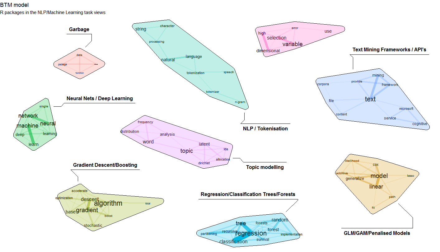
The update which was pushed to CRAN a few weeks ago now allows to explicitely provide a set of biterms to cluster upon. Let us show an example on clustering a subset of R package descriptions on CRAN. The resulting cluster visualisation looks like this.

If you want to reproduce this, the following snippets show how to do this. Steps are as follows

1. Get some data of R packages and their description in plain text

## Get list of packages in the NLP/Machine Learning Task Views
library(ctv)
pkgs <- available.views()
names(pkgs) <- sapply(pkgs, FUN=function(x) x$name)
pkgs <- c(pkgs$NaturalLanguageProcessing$packagelist$name, pkgs$MachineLearning$packagelist$name)

## Get package descriptions of these packages
library(tools)
x <- CRAN_package_db()
x <- x[, c("Package", "Title", "Description")]
x$doc_id <- x$Package
x$text   <- tolower(paste(x$Title, x$Description, sep = "\n"))
x$text   <- gsub("'", "", x$text)
x$text   <- gsub("<.+>", "", x$text)
x        <- subset(x, Package %in% pkgs)

2. Use the udpipe R package to perform Parts of Speech tagging on the package title and descriptions and use udpipe as well for extracting cooccurrences of nouns, adjectives and verbs within 3 words distance.

library(udpipe)
library(data.table)
library(stopwords)
anno    <- udpipe(x, "english", trace = 10)
biterms <- as.data.table(anno)
biterms <- biterms[, cooccurrence(x = lemma,
                                  relevant = upos %in% c("NOUN", "ADJ", "VERB") & 
                                             nchar(lemma) > 2 & !lemma %in% stopwords("en"),
                                  skipgram = 3),
                   by = list(doc_id)]

3. Build the biterm topic model with 9 topics and provide the set of biterms to cluster upon

library(BTM)
set.seed(123456)
traindata <- subset(anno, upos %in% c("NOUN", "ADJ", "VERB") & !lemma %in% stopwords("en") & nchar(lemma) > 2)
traindata <- traindata[, c("doc_id", "lemma")]
model     <- BTM(traindata, biterms = biterms, k = 9, iter = 2000, background = TRUE, trace = 100)

4. Visualise the biterm topic clusters using the textplot package available at https://github.com/bnosac/textplot. This creates the plot show above.

library(textplot)
library(ggraph)
plot(model, top_n = 10,
     title = "BTM model", subtitle = "R packages in the NLP/Machine Learning task views",
     labels = c("Garbage", "Neural Nets / Deep Learning", "Topic modelling", 
                "Regression/Classification Trees/Forests", "Gradient Descent/Boosting", 
                "GLM/GAM/Penalised Models", "NLP / Tokenisation",
                "Text Mining Frameworks / API's", "Variable Selection in High Dimensions"))

Enjoy!