If you are into large data and work a lot with package ff

The ff package is a great and efficient way of working with large datasets.
One of the main reasons why I prefer to use it above other packages that allow working with large datasets is that it is a complete set of tools.
When comparing it to the other open source 'bigdata' packages in R
- It is not restricted to work basically with numeric data matrices like the bigmemory set of packages but allows relatively easy access to character vectors through factors
- It has efficient data loading functionality from flat/csv files, you can interact with SQL databases as explained here.
- You don't need to use the sqldf package to get and insert all the time your data in the right (RAM-limited) sized to and from an SQLite database
- It has higher level functionality (e.g. apply set of family, sorting, ...) which package mmap seems to be lacking
- And it allows you to work with datasets which you can not put in memory which the datatable package does not allow.
If you disagree, do comment.
In my dayly work, I encountered frequently that some bits are still missing in package ff to make it suited for easy day-to-day analysis of large data. Apparently I was not alone as Edwin de Jonge started already package ffbase (available at http://code.google.com/p/fffunctions/). For a predictive modelling project BNOSAC has made for https://additionly.com/ we have made some nice progress in the package.
The package ffbase now contains quite some extensions that are really usefull. It contains a lot of the functionality from the R's base package for usage with large datasets through package ff.
Namely
- Basic operations (c, unique, duplicated, ffmatch, ffdfmatch, %in%, is.na, all, any, cut, ffwhich, ffappend, ffdfappend)
- Standard operators (+, -, *, /, ^, %%, %/%, ==, !=, <, <=, >=, >, &, |, !) on ff vectors
- Math operators (abs, sign, sqrt, ceiling, floor, trunc, round, signif, log, log10, log2, log1p, exp, expm1, acos, acosh, asin, asinh, atan, atanh, cos, cosh, sin, sinh, tan, tanh, gamma, lgamma, digamma, trigamma)
- Selections & data manipulations (subset, transform, with, within, ffwhich)
- Summary statistics (sum, min, max, range, quantile, hist)
- Data transformations (cumsum, cumprod, cummin, cummax, table, tabulate, merge, ffdfdply)
These functions work all on either ff objects or objects of class ffdf from the ff package
Next to that there are some extra goodies allowing faster grouping by - not restricted to the ff package alone (Fast groupwise aggregations: bySum, byMean, binned_sum, binned_sumsq, binned_tabulate)
This makes it a lot more easy to work with the ff package and large data.
Let me show some R-code to show what this means using a simple dataset of the Heritage Health Prize competition of only 2.6Mio records available for download for download here (http://www.heritagehealthprize.com/c/hhp/data). It is a dataset with claims.
The code is for objects of ff/ffdf class and is based on version 0.6 of the package for download here.
require(ffbase)
hhp <- read.table.ffdf(file="/home/jan/Work/RForgeBNOSAC/github/RBelgium_HeritageHealthPrize/Data/Claims.csv", FUN = "read.csv", na.strings = "")
class(hhp)
[1] "ffdf"
dim(hhp)
[1] 2668990 14
str(hhp[1:10,])
'data.frame': 10 obs. of 14 variables:
$ MemberID : int 42286978 97903248 2759427 73570559 11837054 45844561 99829076 54666321 60497718 72200595
$ ProviderID : int 8013252 3316066 2997752 7053364 7557061 1963488 6721023 9932074 363858 6251259
$ Vendor : int 172193 726296 140343 240043 496247 4042 265273 35565 293107 791272
$ PCP : int 37796 5300 91972 70119 68968 55823 91972 27294 64913 49465
$ Year : Factor w/ 3 levels "Y1","Y2","Y3": 1 3 3 3 2 3 1 1 2 3
$ Specialty : Factor w/ 12 levels "Anesthesiology",..: 12 5 5 6 12 10 11 2 11 5
$ PlaceSvc : Factor w/ 8 levels "Ambulance","Home",..: 5 5 5 3 7 5 5 5 5 5
$ PayDelay : Factor w/ 163 levels "0","10","101",..: 52 76 29 48 51 49 40 53 67 82
$ LengthOfStay : Factor w/ 10 levels "1 day","2- 4 weeks",..: NA NA NA NA NA NA NA NA NA NA
$ DSFS : Factor w/ 12 levels "0- 1 month","10-11 months",..: 11 10 1 8 7 6 1 1 4 10
$ PrimaryConditionGroup: Factor w/ 45 levels "AMI","APPCHOL",..: 26 26 21 21 10 26 38 33 19 22
$ CharlsonIndex : Factor w/ 4 levels "0","1-2","3-4",..: 1 2 1 2 2 1 1 1 1 2
$ ProcedureGroup : Factor w/ 17 levels "ANES","EM","MED",..: 3 2 2 7 2 2 3 5 2 7
$ SupLOS : int 0 0 0 0 0 0 0 0 0 0
## Some basic showoff
result <- list()
## Unique members, Unique combination of members and health care providers, find unexpected duplicated records
result$members <- unique(hhp$MemberID)
result$members.providers <- unique(hhp[c("MemberID","ProviderID")])
sum(duplicated(hhp[c("MemberID","ProviderID","Year","DSFS")]))
[1] 936859
## c operator
sum(duplicated(c(result$members, result$members))) # == length(result$members)
[1] 113000
## Basic example of operators is.na.ff, the ! operator and sum.ff
sum(!is.na(hhp$LengthOfStay))
[1] 71598
sum(is.na(hhp$LengthOfStay))
[1] 2597392
## all and any
any(is.na(hhp$LengthOfStay))
[1] TRUE
all(!is.na(hhp$PayDelay))
[1] TRUE
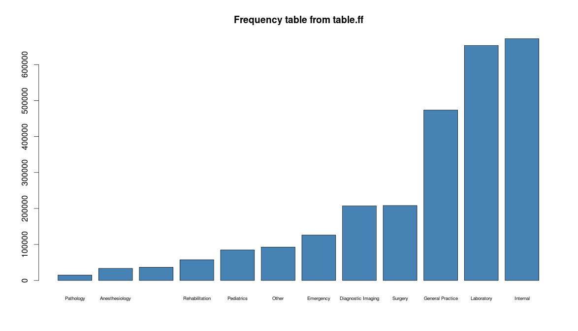
## Frequency table of Specialities and example of a 2-way table
result$speciality <- table.ff(hhp$Specialty, exclude=NA)
options(scipen = 1)
barplot(result$speciality[order(result$speciality)], col = "steelblue", horiz = FALSE, cex.names=0.6, main="Frequency table")
hhp$ProviderFactor <- with(data=hhp[c("ProviderID")], expr = as.character(ProviderID))
result$providerspeciality <- table.ff(hhp$Specialty, hhp$ProviderFactor, exclude=NA)
## Let's see if the member id's are uniformly distributed
hist(hhp$MemberID, col = "steelblue", main = "MemberID's histogram", xlab = "MemberID")
## %in% operator is overloaded
hhp$gp.laboratory <- hhp$Specialty %in% ff(factor(c("General Practice","Laboratory")))
hhp$gp.laboratory
ff (open) logical length=2668990 (2668990)
[1] [2] [3] [4] [5] [6] [7] [8]
FALSE FALSE FALSE TRUE FALSE FALSE FALSE FALSE
[2668983] [2668984] [2668985] [2668986] [2668987] [2668988] [2668989]
: FALSE TRUE FALSE FALSE FALSE FALSE FALSE
[2668990]
FALSE
## Some data cleaning
hhp$pdelay <- with(hhp[c("PayDelay")], as.numeric(PayDelay))
## Summary stats
mean(hhp$pdelay)
[1] 59.78436
range(hhp$pdelay)
[1] 1 163
quantile(hhp$pdelay)
0% 25% 50% 75% 100%
1 45 55 73 163
## cumsum
hist(cumsum.ff(hhp$pdelay), col = "steelblue")
max(cumsum.ff(hhp$pdelay))
[1] 159556245
## cut
table.ff(cut(hhp$pdelay, breaks = c(-Inf, 1, 10, 100, +Inf)), exclude=NA)
(-Inf,1] (1,10] (10,100] (100, Inf]
141451 46720 2237723 243096
## apply a function to a group of data - ddply type of logic from package plyr
hhp$MemberIDFactor <- with(data=hhp[c("MemberID")], expr = as.character(MemberID))
require(doBy)
result$delaybyperson <- ffdfdply(hhp[c("MemberID","pdelay")], split = hhp$MemberIDFactor, FUN=function(x){
summaryBy(pdelay ~ MemberID, data=x, FUN=sum, keep.names=FALSE)
}, trace=FALSE)
result$delaybyperson[1:5,]
MemberID pdelay.sum
1 18190 3158
2 20072 4915
3 20482 4189
4 21207 2548
5 32317 1064
## merging (in fact joining based on ffmatch or ffdfmatch)
hhp <- merge(hhp, result$delaybyperson, by = "MemberID", all.x=TRUE, all.y=FALSE)
names(hhp)
[1] "MemberID" "ProviderID" "Vendor"
[4] "PCP" "Year" "Specialty"
[7] "PlaceSvc" "PayDelay" "LengthOfStay"
[10] "DSFS" "PrimaryConditionGroup" "CharlsonIndex"
[13] "ProcedureGroup" "SupLOS" "ProviderFactor"
[16] "gp.laboratory" "pdelay" "MemberIDFactor"
[19] "pdelay.sum"
## Let's add a key (in version 0.6 of the package for download here)
hhp$key <- key(hhp[c("MemberID","ProviderID")])
max(hhp$key) == nrow(result$members.providers)
[1] TRUE
## A small example of operators
idx <- ffwhich(hhp[c("Specialty","PlaceSvc")], Specialty == "General Practice")
idx
ff (open) integer length=473655 (473655)
[1] [2] [3] [4] [5] [6] [7] [8]
18 19 20 31 35 42 45 62
[473648] [473649] [473650] [473651] [473652] [473653] [473654]
: 2668922 2668929 2668930 2668947 2668952 2668965 2668974
[473655]
2668984
hhp.gp <- hhp[idx, ]
class(hhp.gp)
[1] "ffdf"
nrow(hhp.gp)
[1] 473655
sum(is.na(idx))
[1] 0
sum(hhp$Specialty == "General Practice", na.rm=TRUE)
[1] 473655
## Or apply subset
table.ff(hhp$Year, exclude=NA)
Y1 Y2 Y3
865689 898872 904429
hhp.y1 <- subset(hhp, hhp$Year == "Y1")
nrow(hhp.y1)
[1] 865689
We welcome you to use the package if it suits your applications and if you have any requests, do post some comments to see how the package can be extended for your needs.