Advanced R programming topics
Similarly as last year, BNOSAC is offering the short course on 'Advanced R programming topics' at the Leuven Statistics Research Center (Belgium).
The course is now part of FLAMES (Flanders Training Network for Methodology and Statistics) and can be found here http://www.flames-statistics.eu/training/advanced-r-programming-topics. Subscription is no longer possible unless you ask kindly to LStat.
RApache and developing web applications with R as backend
As the demand of courses on R is increasing, we are thinking also about giving a course on RApache and developing web applications with R as a backend. This course will allow you to build applications like this one http://rweb.stat.ucla.edu/lme4/ or this one http://rweb.stat.ucla.edu/ggplot2/.
BNOSAC has quite some (private) business applications running involving this technology stack and would to share with you it's knowledge. If you are interested in these courses which combine javascript, R and RApache, get in contact with us and send a mail by filling out the form at index.php/contact/get-in-touch. The more people interested, the lower the cost of the course ... .

Myrrix is probably more known by java developers and users of Mahout than R users. This is because most of the times java and R developers live in a different community.
If you go to the website of Myrrix (
http://myrrix.com), you'll find out that it is a
large-scale recommender system which is able to build a recommendation model based on Alternating Least Squares. That technique is a pretty good benchmark model if you tune it well enough to get recommendations to your customers.
It has a setup which allows you to build recommendation models with local data and a setup to build a recommender system based on data in Hadoop - be it on
CDH or on another Hadoop stack like
HDInsights or your own installation.
Very recently, Cloudera has shown the intention to incorporate Myrrix into it's product offering (
see this press release) and this is getting quite some attention.
Recommendation engines are one of the techniques in machine learning which get frequent attention although they are not so frequently used as other statistical techniques like classification or regression.
This is because a recommendation engines most of the time require a lot of processing like deciding on which data to use, handling time-based information, handling new products and products which are no longer sold, making sure the model is up-to-date andsoforth.
When setting up a recommendation engine, business users also want to compare their behaviour to other business-driven or other data-driven logic. In these initial phases of a project, allowing statisticians and data scientists to use their language of choice to communicate with, test and evaluate the recommendation engine is key.
To allow this, we have created an
interface between R and Myrrix, containing 2 packages which are currently available on github (
https://github.com/jwijffels/Myrrix-R-interface). It allows R users to build, finetune and evaluate the recommendation engine as well as retrieve recommendations. Future users of Cloudera might as well be interested in this, once Myrrix gets incorporated into their product offering.
Myrrix deploys a recommender engine technique based on large, sparse matrix factorization. From input data, it learns a small number of "features" that best explain users' and items' observed interactions. This same basic idea goes by many names in machine learning, like principal component analysist or latent factor analysis. Myrrix uses a modified version of an Alternating Least Squares algorithm to factor matrices. More information can be found here:
http://www.slideshare.net/srowen/big-practical-recommendations-with-alternating-least-squares and at the
Myrrix website.
So if you are interested in setting up a recommendation engine for your application or if you want to improve your existing recommendation toolkit,
contact us.If you are an R user and only interested in the code on how to build a recommendation model and retrieve recommendations, here it is. The packages will be pushed to CRAN soon.
# To start up building recommendation engines, install the R packages Myrrixjars and Myrrix as follows.

install.packages("devtools")
install.packages("rJava")
install.packages("ffbase")
library(devtools)
install_github("Myrrix-R-interface", "jwijffels", subdir="/Myrrixjars/pkg")
install_github("Myrrix-R-interface", "jwijffels", subdir="/Myrrix/pkg")

## The following example shows the basic usage on how to use Myrrix to build a local recommendation
## engine. It uses the audioscrobbler data available on the Myrrix website.

library(Myrrix)
## Download example dataset
inputfile <- file.path(tempdir(), "audioscrobbler-data.subset.csv.gz")
download.file(url="http://dom2bevkhhre1.cloudfront.net/audioscrobbler-data.subset.csv.gz", destfile = inputfile)

## Set hyperparameters
setMyrrixHyperParameters(params=list(model.iterations.max = 2, model.features=10, model.als.lambda=0.1))
x <- getMyrrixHyperParameters(parameters=c("model.iterations.max","model.features","model.als.lambda"))
str(x)

## Build a model which will be stored in getwd() and ingest the data file into it
recommendationengine <- new("ServerRecommender", localInputDir=getwd())
ingest(recommendationengine, inputfile)
await(recommendationengine)

## Get all users/items and score alongside the recommendation model
items <- getAllItemIDs(recommendationengine)
users <- getAllUserIDs(recommendationengine)
estimatePreference(recommendationengine, userID=users[1], itemIDs=items[1:20])
estimatePreference(recommendationengine, userID=users[10], itemIDs=items)
mostPopularItems(recommendationengine, howMany=10L)
recommend(recommendationengine, userID=users[5], howMany=10L)
A few weeks ago, Rstudio released it's download logs, showing who downloaded R packages through their CRAN mirror. More info: http://blog.rstudio.org/2013/06/10/rstudio-cran-mirror/
This is very nice information and it can be used to show the popularity of packages with R, which has been done
before and
criticized also as the RStudio logs might/might not be representative for the download behaviour of all useRs.
As the
useR2013 conference has come to an end, one of the topics corporate useRs of R seem to be talking about is how to speed up R and how R handles large data.
Edwin & BNOSAC did their fair share by giving a presentation about the use of
ffbase alongside the
ff package which can be found
here 
.
When looking at twitter feeds (
https://twitter.com/search?q=user2013), there is now Tibco who has it's own R interpreter, there is R inside the JVM, Rcpp, Revolution R, ff/ffbase, R inside Oracle, there is pbdR, pretty quick R (pqR), MPI, R on grids, R with mongo/monet-DB, PL/R, dplyr and useRs made a lot of presentations about how they handled large data in their business setting. It seems like the use of R with large datasets is being more and more accepted in the corporate world - which is a good thing. And we love the diversity!
For R packages which are on CRAN, the Rstudio download logs can be used to show download statistics of the open source bigdata / large data packages which are now on the market (CRAN).
For this, the logs were downloaded and a number of open source packages which are out-of-memory / bigdata solutions in R were compared with respect to download stats on this mirror.
It seems like by far the most popular package is ff and our own contribution (ffbase) is not doing bad at all (+/- 100 ip addresses downloaded our package per week from the Rstudio CRAN mirror only).
If you are interested in the code to download the data and get the plot or if you want to compare your own packages, you can use the following code.
##
## Rstudio logs
##
input <- list()
input$path <- getwd()
input$path <- "/home/janw/Desktop/ffbaseusage"
input$start <- as.Date('2012-10-01')
input$today <- as.Date('2013-06-10')
input$today <- Sys.Date()-1
input$all_days <- seq(input$start, input$today, by = 'day')
input$all_days <- seq(input$start, input$today, by = 'day')
input$urls <- paste0('http://cran-logs.rstudio.com/',
                     as.POSIXlt(input$all_days)$year + 1900, '/', input$all_days, '.csv.gz')
##
## Download
##
sapply(input$urls, FUN=function(x, path) {
  print(x)
  try(download.file(x, destfile = file.path(path, strsplit(x, "/")[[1]][[5]])))
}, path=input$path)

##
## Import the data in a csv and put it in 1 ffdf
##
require(ffbase)
files <- sort(list.files(input$path, pattern = ".csv.gz$"))
rstudiologs <- NULL
for(file in files){
  print(file)
  con <- gzfile(file.path(input$path, file))
  x <- read.csv(con, header=TRUE, colClasses = c("Date","character","integer", rep("factor", 6), "numeric"))
  x$time <- as.POSIXct(strptime(sprintf("%s %s", x$date, x$time), "%Y-%m-%d %H:%M:%S"))
  rstudiologs <- rbind(rstudiologs, as.ffdf(x))
}
dim(rstudiologs)
rstudiologs <- subset(rstudiologs, as.Date(time) >= as.Date("2012-12-31"))
ffsave(rstudiologs, file = file.path(input$path, "rstudiologs"))


library(ffbase)
library(data.table)
tmp <- ffload(file.path(input$path, "rstudiologs"), rootpath = tempdir())
rstudiologs[1:2, ]
packages <- c("ff","ffbase","bigmemory","mmap","filehash","pbdBASE","colbycol","MonetDB.R")
idx <- rstudiologs$package %in% ff(factor(packages))
idx <- ffwhich(idx, idx == TRUE)
mypackages <- rstudiologs[idx, ]
mypackages <- as.data.frame(mypackages)
info <- c("r_version","r_arch","r_os","package","version","country")
mypackages[info] <- apply(mypackages[info], MARGIN=2, as.character)
mypackages <- as.data.table(mypackages)
mypackages$aantal <- 1
mondayofweek <- function(x){
    weekday <- as.integer(format(x, "%w"))
    as.Date(ifelse(weekday == 0, x-6, x-(weekday-1)), origin=Sys.Date()-as.integer(Sys.Date()))
  }
mypackages$date <- mondayofweek(mypackages$date)
byday <- mypackages[,
                    list(aantal = sum(aantal),
                         ips = length(unique(ip_id))),
                    by = list(package, date)]
byday <- subset(byday, date != max(as.character(byday$date)))

library(ggplot2)
byday <- transform(byday, package=reorder(package, byday$ips))
qplot( data=byday, y=ips, x=date, color=reorder(package, -ips, mean), geom="line", size=I(1)
) + labs(x="", y="# unique ip", title="Rstudio logs 2013, downloads/week", color="") + theme_bw()
A few weeks ago, the stream package has been released on CRAN. It allows to do real time analytics on data streams. This can be very usefull if you are working with large datasets which are already hard to put in RAM completely, let alone to build some statistical model on it without getting into RAM problems.
Most of the standard statistical algorithms require access to all data points and make several iterations over the data and are less suited for usage in R on big datasets.
Streaming algorithms on the other hand are characterised by
- single passes over the data,
- using a limited amount of storage space and RAM
- work in a limited amount of time
- be ready to use the model at any time
The stream package is currently focussed on clustering algorithms available in MOA (
http://moa.cms.waikato.ac.nz/details/stream-clustering/) and also eases interfacing with some clustering already available in R which are suited for data stream clustering. Classification algorithms based on
MOA are on the todo list.
Current available clustering algorithms are BIRCH, CluStream, ClusTree, DBSCAN, DenStream, Hierarchical, Kmeans and Threshold Nearest Neighbor.
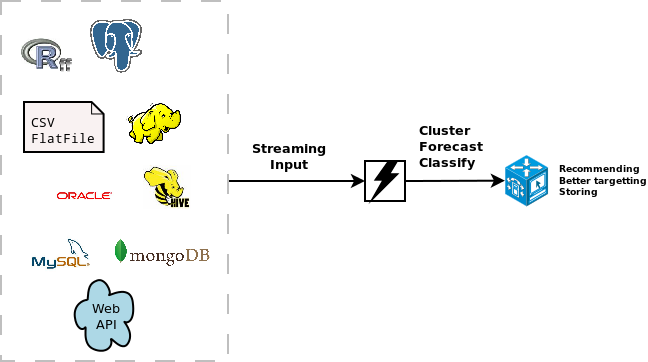
The stream package allows you to
easily extend the use of the models with different data sources. These can be SQL sources, Hadoop, Storm, Hive, simple csv files, flat files or other connections. It is quite easy to extend it towards other connections. As an example, the following code available at this gist (
https://gist.github.com/jwijffels/5239198) allows it to connect to an
ffdf from the
ff package.
This allows to do clustering on ff objects.
Below, you can find a toy example showing streaming clustering in R based on data in an ffdf.
- Load the packages & the Data Stream Data for ffdf objects
require(devtools)
require(stream)
require(ff)
source_gist("5239198")
myffdf <- as.ffdf(iris)
myffdf <- myffdf[c("Sepal.Length","Sepal.Width","Petal.Length","Petal.Width")]
mydatastream <- DSD_FFDFstream(x = myffdf, k = 100, loop=TRUE)
mydatastream
- Build the streaming clustering model
#### Get some points from the data stream
get_points(mydatastream, n=5)
mydatastream
#### Cluster (first part)
myclusteringmodel <- DSC_CluStream(k = 100)
cluster(myclusteringmodel, mydatastream, 1000)
myclusteringmodel
plot(myclusteringmodel)
#### Cluster (second part)
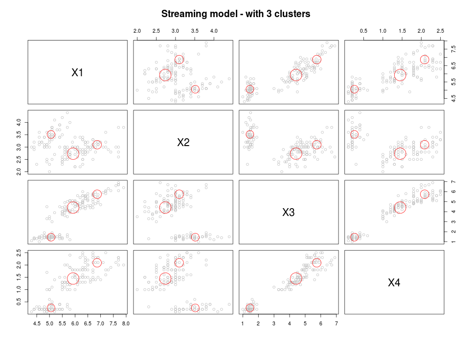
kmeans <- DSC_Kmeans(3)
recluster(kmeans, myclusteringmodel)
plot(kmeans, mydatastream, n = 150, main = "Streaming model - with 3 clusters")
This approach is a standard 2-step approach which combines streaming micro clustering with macro clustering using a basic kmeans algorithm.